Main Menu
- Home
- Product Finder
- Calibration Systems
- Calibration Services
- Digital Sensing
- Industrial Vibration Calibration
- Modal and Vibration Testing
- Non-Destructive Testing
- Sound & Vibration Rental Program
- Learn
- About Us
- Contact Us
 Often accelerometers are treated as a “black box” with little regard to the internal structure or function. The wide spread integration of built-in ICP® sensor power into most modern day dynamic
data acquisition systems often places two wire, constant current signal conditioning in this “black box” domain as well. As a result, many users have requested more information on the structure and performance of dynamic sensors.
Often accelerometers are treated as a “black box” with little regard to the internal structure or function. The wide spread integration of built-in ICP® sensor power into most modern day dynamic
data acquisition systems often places two wire, constant current signal conditioning in this “black box” domain as well. As a result, many users have requested more information on the structure and performance of dynamic sensors.
Accelerometers serve to measure motion or vibration by converting physical movement into an electrical signal suitable for measurement, recording, analysis and/or control. To do its job, the ideal behavior of an accelerometer is actually very simple – straight lines! This means that the accelerometer exhibits a flat amplitude sensitivity and phase response with respect to frequency, and straight-line amplitude linearity. (Click here to read a classic 1-page paper about transduction).
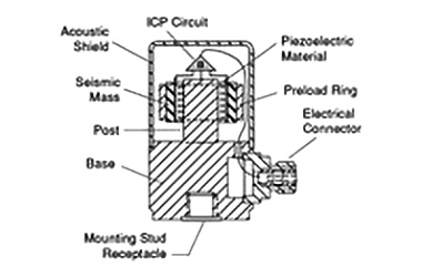
To achieve this ideal behavior, accelerometer manufacturers employ various structures usually composed of an inertial mass deflecting some type of beam or crystal for the internal sensing element. The sensing crystal is extremely stiff with a modulus of 15E6 psi (104E9 N/m2), on the order of stainless steel, and exhibits virtually no deflection during the measurement process. This allows for both excellent long term durability (near solid state performance) and also allows for a high natural frequency/broad frequency operating range. (Click here for more on General Piezoelectric Theory). Typical internal mechanical configurations include compression, inverted compression, shear and flexural/beam. These internal configurations can often be represented mechanically as a simple spring-mass system exhibiting the response of a single degree-of-freedom second order system.
Accordingly, the sensing elements will have certain ranges where the output behavior performs nearly ideal. As such, there is a specified frequency range where the amplitude frequency response is essentially flat (typical specified as +/- 5%). The low frequency end of this range is governed electrically by the coupling and time constant of the sensor and signal conditioning, while the high frequency end of the this range is governed mechanically by the resonant frequency (fn) and associate damping (ζ) of the mounted sensor. (Click here to read a classic 1-page paper on signal conditioning). Verifying the straight-line behavior of these various designs, as well as determining the proper scaling factor or “calibration value” is the province of the metrology lab.